Satellite observation of glaciers | Mapping structural glaciology | Mapping glacier change | Mapping glacier thinning | Mapping glacier velocity | Other glaciological applications | Different satellites with different capabilities | Summary and conclusions | Further reading | References | Comments |
Satellite observation of glaciers

Ice cover on Earth is changing. We have records going back decades, measuring the mass balance of glaciers in the Alps. We can measure the distance between the modern glacier terminus and its maximum position during the Little Ice Age, around 1850 AD in the northern hemisphere. We can visit the same glacier each year for ten years and visually see the recession of its snout. However, empirical field measurements of glacier mass balance and recession are arduous, time consuming and expensive. Point measurements are collected from just a small number of reference glaciers. But the advent of remote sensing over the last 40 years has opened up unparalleled opportunities for glacier observation.
Cameras in space

“Remote Sensing” just means the acquisition of information about an object without touching it. We have been “remote sensing” with our eyes for millennia. But put a camera up into space, and suddenly, we can observe glacier behaviour at a much larger scale. With repeated images over time, we can easily see how glaciers have changed.
“Remote sensing” includes obtaining information from aerial photographs from drones or aeroplanes, multibeam swath bathymetry data from ships, ground penetrating radar data and more. In this article, we focus only on remote sensing from satellites.
Earth Observation satellites orbit the Earth, taking pictures in various bands of the electromagnetic spectrum, from visible to thermal infrared. The large swaths (footprint of the image on the ground) make regional assessments simple. Each satellite takes pictures at a different resolution, and so each is used for different applications. Optical satellite remote sensing allows for the regular monitoring of glacier surface elevation, velocity, area, length, equilibrium line altitude, terminus position and more1,2.
Hundreds of applications for remote sensing

Remote sensing is a mature technique with many applications. The following gives some examples of how satellite imagery and remote sensing is used in the world of glaciology. Feel free to add a Comment and tell us how you use remote sensing in your glaciological research!
Scroll to the Different satellites with different capabilities section to find out all about each of the different satellites that glaciologists use for remote sensing of cryospheric change.
Mapping structural glaciology

Satellites providing visual images of Earth are great for mapping regional glacier and ice-shelf structures. ASTER and Landsat images are frequently used for this kind of work, because their large swaths (footprint) means that a regional view of the ice is provided, but their relatively fine resolution means that even small glacier structures, such as crevasses and melt ponds, can be imaged and mapped. The long time series of images from these satellites (ASTER since 1999, Landsat since the 1970s), is useful for mapping changes over time.
Larsen B Ice Shelf

As an example, Glasser and Scambos used optical satellite imagery (ASTER and Landsat 7) to map detailed changes in ice structures in the build-up to the collapse of Larsen B ice shelf in 2002. Their maps showed rifts becoming more pronounced in the years before the ice-shelf collapse, and that ice-shelf collapse was preconditioned by partial rupturing of the sutures between flow units3. This shows one of the great advantages of satellite remote sensing – after a catastrophic event, such as ice-shelf collapse, you can go back in time and analyse how the ice behaved prior to disintegration.
Prince Gustav Ice Shelf

The situation is similar for Prince Gustav Ice Shelf, where the ice shelf suture zones formed zones of weakness, abetting ice-shelf collapse4, which occurred in 1995. The Landsat image opposite shows clear sutures forming between flow units. Meltwater ponding on the surface eventually aided iceberg formation and ice-shelf disintegration by melting rapidly downwards through the ice shelf.
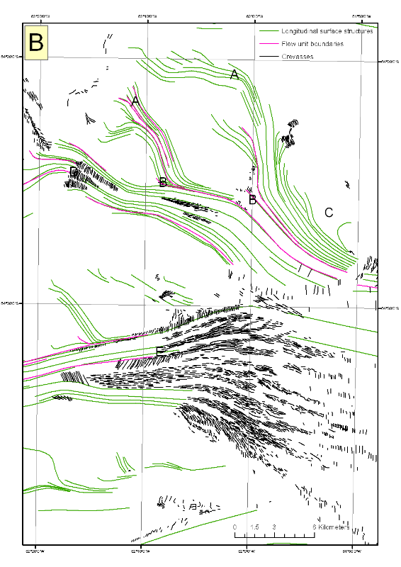
Ice shelves on the SW Antarctic Peninsula
Holt et al. also used Landsat images to map the surface features of ice shelves on the south-western Antarctic Peninsula. Tom Holt was able to map the ice front, grounding zone, longitudinal surface structures (flow stripes), pressure ridges, crevasses, fractures and rifts, surface meltwater, ice dolines, ice rises and ice rumples5. Together, these data help us to understand the structure of more ‘stable’ ice shelves, and helps us to assess their likely future response and vulnerabilities to climate change6.

Flow stripes on Antarctic ice streams
Glasser and Gudmundsson (2012) have mapped surface structures on a number of Antarctic ice streams7. Because the pattern of velocity varies across the ice streams, crevasses and flow lines form.


Mapping glacier change
Glacier recession in Patagonia

Because of the long history of optical satellite imagery of the Earth, satellite remote sensing offers fabulous opportunities for mapping glacier recession. It is simple to derive 40+ year histories of regional glacier recession8-11. Landsat and ASTER images are frequently used for this application. For example, remote sensing of glacier ice and Little Ice Age moraines in Patagonia (formed circa 1870) and glacier extent in 2011, 2001, 1986 and 1975 provides a detailed analysis of rates of recession over the last 140 years12.

Conducting glacier inventories
Glacier inventories are also an essential part of glaciological monitoring, and many parameters, such as glacier length, altitudinal range, snow cover and so on can be calculated from satellite images. These data are essential for wider studies and modelling of glaciers. The GLIMS Geospatial Database13 provides detailed guidelines on the correct methods for conducting glacier inventories14-19, and a free online database where any user can download outlines of all inventoried glaciers.
Additional data often mapped by satellite and added to glacier inventories include changing ice debris cover20, rock glaciers21, equilibrium line altitude22, grounding zones23 and glacial lake extent24,25. Volume-area scaling laws mean that you can calculate changing ice volume26. The applications are as limitless as your imagination.
Mapping glacier thinning
While it’s important to map glacier recession, it’s not the whole story. Glaciers may be thinning and downwasting in situ, with little change at their terminus. Mapping glacier thinning is therefore an important application of glacier remote sensing. One way of doing this is to generate two digital elevation models from two different time periods and to subtract one from the other (e.g., ref. 27). However, this isn’t easy as it assumes that the change in surface elevation is greater than the errors and uncertainties in the digital elevation models.
Dynamic thinning around Pine Island Glacier and the Antarctic Peninsula
One analysis by Kunz et al. of images taken from aeroplanes (1948-2005) and ASTER stereo-pairs (2001-2010) showed that glaciers in the western Antarctic Peninsula have been thinning over the last few decades28. All the glaciers show surface lowering in their ablation zones since the 1960s, with the highest rates of thinning occurring in the north-western Antarctic Peninsula region28.
Another method of calculating elevation change is to use ICESat data. This satellite measures ice surface elevation, and repeated tracks show elevation change through time. Analysis of ICESat data across George VI Ice Shelf on the south-western Antarctic Peninsula agreed with the DEM differencing work conducted by Kunz et al. Holt et al. analysed surface elevation change of George VI Ice Shelf using ICESat’s GLAS repeat measurements from 2003 to 20086. Significant thinning was observed in the southern section of the ice shelf, which is coupled with widespread recession of the ice front terminus.


Thinning ice shelves

(Pritchard et al. 2012), copyright (2012).
ICESat has also been used to calculate ice-shelf thinning and basal melt in ice shelves around Antarctica30. Pritchard et al. used a combination of satellite laser altimetry and modelling of the surface firn layer to show ice-shelf thinning around Antarctica as a result of increased basal melt. This melt is the primary control on Antarctic ice-sheet loss, as the thinner ice shelves are less able to buttress ice in the interior, leading to faster ice flow. The strongest thermal forcing and highest melt rates were found near Pine Island Glacer, West Antarctica.
Mapping glacier velocity
Measuring regional glacier and ice stream velocity, and its change through time, is a critical application of glacier remote sensing. There are several methods; the first relies on repeated optical satellite imagery of one region. An algorithm applied to the images calculates the distance that features on the ice surface have moved (feature tracking) (e.g., 27). Cosi-Corr is frequently used for feature tracking in this way31,32. A second method uses repeat radar images (Synthetic Aperture Radar interferometry, or InSAR) to calculate glacier velocity. Two pairs of images are used to calculate ascending-pass and descending-pass interferograms. Velocity fields can then be calculated6.
Ice velocity on George VI Ice Shelf
For example, Tom Holt used a combination of radar and optical feature tracking to examine the response of George VI Ice Shelf to environmental change6. This analysis showed ice-shelf acceleration towards the north and south ice fronts, combined with thinning throughout and an increase in fracture distribution towards the southern ice front.

Mapping Antarctic ice stream velocity

Eric Rignot compiled masses of InSAR velocity data to present a comprehensive, high resolution map of Antarctic ice velocity. The data revealed widespread enhanced flow, with tributary glaciers reaching deep into the ice-sheet’s interior.
Other glaciological applications
There are many hundreds of applications of remote sensing data for glaciers, so I will just pick out a few here.
Mapping Equilibrium Line Altitudes
Glacier inventory data (information on glacier length, altitudinal range, thickness, snow cover etc) can be used to calculate regional Equilibrium Line Altitudes (ELAs)22. These data provide important information on glacier mass balance, an important glaciological parameter.
Mapping snow cover
Related to above is mapping of snow cover. This has important applications for understanding glacier mass balance as well as the behaviour of perennial snow patches, water resources and more. Scientists may set up algorithms to automatically classify terrain with different reflectance values (white snow, dark water, green land etc). This makes it simple to quickly map changing snow cover in a wider region.
Mapping glacier landforms
Glacial geology has been revolutionised by satellite remote sensing. Large swaths mean that images that are subtle and difficult to map on the ground can be quickly and easily mapped from space. A typical example is mega-scale glacial lineations; these features have now been recognised in glaciated terrains across the northern hemisphere, and are easily visible in a digital elevation model created from satellite images (e.g., see 33-35).
Measuring the ice-sheet bed
Information on bed topography is one of the key parameters needed to drive ice-sheet and glacier numerical models. Unfortunately, the bed of a glacier is rather difficult to get at. Fortunately, radar mounted on satellites can penetrate the ice, helping to map the geometry of the ground beneath the ice. Synthetic aperture radar (SAR) can be used to generate digital elevation models of the ice bed, even in the most remote of regions36.
Different satellites with different capabilities
There are various satellites used for observation of ice sheets. They have different resolutions (pixel size in the image) and swath sizes (the footprint of the image on the ground). They have different return rates (returning to take the same image). As a result, different applications are best suited to different satellites. ASTER and Landsat are some of the most widely used sensors in glaciology, due to their long history of taking images, broad swaths allowing for regional analysis, and high image resolution. ASTER also takes images as stereo-pairs, meaning that digital elevation models can be made from its images (ASTER GDEM).
Some of the most common satellites used in glacier and ice sheet observation are:
| Satellite name | Ground resolution (pixel size) | Swath size | Operation dates | Sensors | Applications | |
|
Visualising the Earth |
ASTER | 15 m | 60 km | Launched December 1999 | Multispectral (14 bands) sensor. Three separate sensors: VNIR (Visible Near Infrared), (15 m)SWIR (ShortWave Infrared), (30 m)TIR (Thermal Infrared) (90 m) |
ASTER data is used to create detailed maps of land surface temperature, reflectance, and elevation.ASTER captures high spatial resolution data in 14 bands, from the visible to the thermal infrared wavelengths, and provides stereo viewing capability for digital elevation model creation. |
| Landsat 7 ETM+ | 30 m | 185 km | Launched April 1999 | Multispectral (7 bands) | Series of satellites (currently Landsat 8), with the earliest images dating from the 1970s. | |
| Spot-5 | 5 m and 2.5 m | 60 x 60 km and 60 x 120 km | Launched May 2002. | Twin sensors.Multispectral and panchromatic.1 shortwave infrared. | The coverage offered by SPOT-5 is a key asset for applications such as medium-scale mapping (at 1:25 000 and 1:10 000 locally). Revisit time: 2-3 days | |
| ENVI Sat | 30 m | 58 km | March 2002 to May 2012. | Multispectral with synthetic aperture radar. | Repeat cycle of 35 days. After losing contact with the satellite on 8 April 2012, ESA formally announced the end of Envisat’s mission on 9 May 2012 | |
| MODIS | 250 m (bands 1-2) 500 m (bands 3-7) 1000 m (bands 8-36) |
2330 km | Launched May 2002. | Multispectral (36 spectral bands) | MODIS (or Moderate Resolution Imaging Spectroradiometer) is a key instrument aboard the Terra (EOS AM) and Aqua (EOS PM) satellites.Terra MODIS and Aqua MODIS are viewing the entire Earth’s surface every 1 to 2 days, acquiring data in 36 spectral bands, or groups of wavelengths | |
| Quickbird | 0.61 m | 16.5 Km x 16.5 Km at nadir | Launched October 2001 | Multispectral | QuickBird is a high resolution satellite owned and operated by DigitalGlobe. This satellite is an excellent source of environmental data useful for analyses of changes in land usage, agricultural and forest climates. | |
| Geo-Eye | 0.41 m panchromatic; 1.65 m multispectral | 15.2 km | Launched September 2008 | Pan-sharpened multispectral imagery. | Revisit time of 3 days. | |
| Worldview-2 | 0.46 m panchromatic; 1.85 m multispectral | 16.4 km | Launched October 2009 | Multispectral (8 bands) | Revisit time of every 1.1 days. | |
|
Measuring elevation change |
Cryosat | 250 m wide strips. | Launched April 2010 | Synthetic Aperture Interferometric Radar Altimeter (SIRAL). The altimeter makes a measurement of the distance between the satellite and the surface. | Cryosat is designed to calculate the elevation of ice and sea-ice ‘freeboard’, which is the height protruding from the water. Its aim is to determine changes in land-ice and sea-ice thickness.It reaches 88°N and S on every orbit. | |
| ICEsat | Can detect changes in elevation of up to 1 cm per year. | 60 m | January 2003-2009. Decommissioned August 2010. ICEsat-2 is planned in 2016. | Lasers for measuring elevation change | Ice, Cloud, and land Elevation Satellite. The ICESat mission provided multi-year elevation data needed to determine ice sheet mass balance as well as cloud property information. ICESat ended its science mission in February 2010 with the failure of the last of its three lasers. | |
| SRTM | 90 m for the DEM | 225 km | February 2000 (single mission) | Radar | The Shuttle Radar Topography Mission (SRTM) obtained elevation data on a near-global scale to generate the most complete high-resolution digital topographic database of Earth. SRTM consisted of a specially modified radar system that flew on-board the Space Shuttle Endeavour during an 11-day mission in February of 2000. | |
|
Measuring gravity |
GRACE | March 2002 | The mission uses a microwave ranging system to accurately measure changes in the speed and distance between two identical spacecraft flying in a polar orbit about 220 kilometres (140 mi) apart, 500 kilometres (310 mi) above Earth. | The Gravity Recovery And Climate Experiment (GRACE). Twin satellites making detailed measurements of the Earth’s gravity field. Changes in the gravity are interpreted in terms of changes to the Earth’s ice sheets. |
Summary and conclusions for remote sensing of glaciers
Satellite remote sensing has revolutionised glaciology and glacial geology by enabling quick, cheap and logistically simple ways to map large landscapes. It has enabled glacier inventories of entire countries, underpinned our understanding of glacier recession and advance, helps us to map glacier snow cover and mass balance, track changes in ice sheet thickness and ice flow velocities, and allowed detailed changes in remote locations to be observed.
Do you have a favourite glacier remote sensing technique? How do you use satellite images in your work? Add in an example in the Comments box and tell us!
Hello,
I am researching the Haut Glacier D’Arolla for my dissertation. Do you know how may I get hold of long term (46yrs) meteorological and mass balance/ablation data for the glacier/Arolla area as well as a debris cover database? Meteorological data from the nearby Grand St Bernard Pass, Bricola and the Evolene weather stations is also greatly appreciated.
I am researching the variable response of the glacier to global warming with differing amounts of debris cover for my degree at the University of Edinburgh.
I would really appreciate any help/advice.
Kind regards,
Natasha Smellie.
Good day,
I am researching on Protection solutions for mountain glacier movement here in Switzerland.
I need to measure a detached glacier data here in Swiss. I need reliable dada provided by satellite.
How can I contact with your technical department.
Thanks
Fredric Bakhtiar , LinkedIn
From Geneva