What is glacier response time? | The role of glacier size | The role of mass balance gradients | The role of glacier slope and hypsometry | Calculating glacier response times | Summary | Further reading | References | Comments |
What is glacier response time?
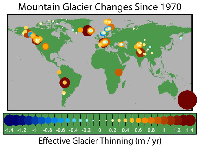
Glacier response time is the length of time taken for a glacier to adjust its geometry to a new steady state after a change in glacier mass balance1, caused by a changing climate2. Mountain glaciers worldwide are currently thinning and receding, but their behaviour in the future is highly variable, as their recession is controlled by many parameters. Understanding glacier response time is important for understanding how quickly particular glaciers will change in length and volume under a given climatic scenario; if we are to be able to estimate future sea level rise from shrinking glaciers, we need to know how quickly they can change2. Will glaciers shrink in response to short term climate fluctuations, or are longer and more sustained climatic changes required before a glacier changes its geometry?
The response time of a glacier is largely a function of its mean thickness and terminus ablation3 (Table 1), and of its hypsometry and mass balance gradient4,5 (the change in accumulation and ablation with elevation; a glacier with a steeper mass balance gradient receives more accumulation and has more ablation than a dry glacier with little accumulation and ablation). High mass balance gradients are indicative of high flux through the ELA. High gradients are usually found in mid-latitude maritime regions, where the maritime environment represents a major heat and moisture source6. Glacier size also affects glacier response time7.

Table 1. Estimated glacier response times as a function of thickness and terminus ablation. From Cuffey and Patterson, 2010.
| Thickness (m) | Terminus ablation (m per year) | Response time (years) | |
| Glaciers in temperate maritime climate | 150-300 | 5-10 | 15-60 |
| Glacier in high-polar climate | 150-300 | 0.5-1 | 150-600 |
| Ice caps in Arctic Canada | 500-1000 | 1-2 | 250-1000 |
| Greenland Ice Sheet | 3000 | 1-2 | 1500-3000 |
The role of glacier size

Smaller glaciers have shorter response times, and this is one of the reasons why small glaciers currently contribute significantly to sea level rise10,11. The high sensitivity of small ice masses to climate change is a function of their small system scale, and their proximity (compared with larger ice sheets) to the melting point9. However, it is difficult to apply a uniform response time widely across multiple glaciers. There is no straightforward relationship between glacier size and change in ice volume under any given climate scenario12.
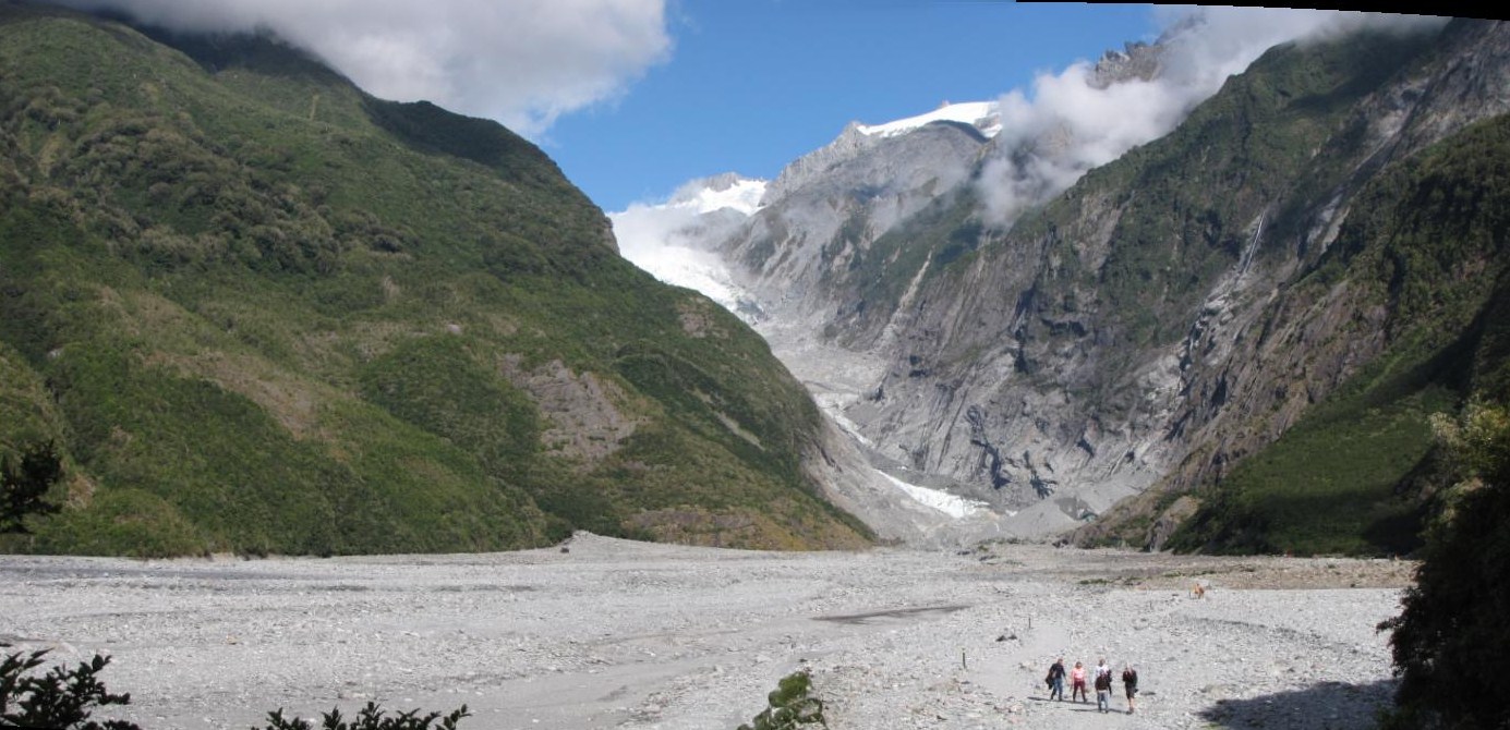
Short, steep glaciers in maritime environments (with a correspondingly steep mass balance gradient) reach equilibrium following a change in mass balance forcing after only a few years, larger valley glaciers in around a century, and continental ice caps with gentle slopes much longer4. The smallest cirque glaciers will reflect annual changes in mass balance, almost without delay8. Franz Josef Glacier, in New Zealand, is 11 km long and 35 km2 in area, has a steep surface gradient and a steep mass balance gradient, and has a response time of 21-24 years9. The Greenland Ice sheet, on the other hand, is estimated to have a response time of 1500-3000 years5.

The implication of this is that, given the same climatic forcing, glaciers of different lengths and thicknesses will respond in different ways, with variable numbers of advances and retreats. These should generally correlate regionally. Moraines occurring at only a few glaciers at a specific time are interpreted as reflecting shorter term climatic oscillations and a glacier with a short response time4. Larger, flatter glaciers tend to smooth the climatic signal, with a delay of several decades.
The role of mass balance gradients

A key factor in controlling glacier response to climatic perturbations is the mass balance gradient, the change in net balance with altitude, which is largely governed by the temperature lapse rate2,6. There is a linear relationship between mass balance gradient and mass balance sensitivity. Glaciers with a steeper mass balance gradient flow faster. The mass balance gradient of a glacier is affected by glacier size, hypsometry (the variation of glacier area with altitude13) and glacier slope.
Wet, maritime glaciers have a steeper mass balance gradient than dry continental glaciers. Warm, wet glaciers with a steep mass balance gradient and high sensitivity have a small response time, and cold and dry glaciers with low mass balance gradients and sensitivity have typically a longer response time. Temperature-sensitive glaciers may show the most rapid response to climate change at present, but may not be the most important contributors to global sea level rise over longer time periods2.
The role of glacier slope and hypsometry
Glacier hypsometry controls the mass balance elevation distribution over a glacier13. Glacier hypsometry is determined by valley shape, topographic relief and ice volume distribution. The altitudinal distribution of a glacier controls its sensitivity to a rise in the Equilibrium Line Altitude (ELA); glaciers with a large, relatively flat accumulation area will be more sensitive to a small increase in ELA than glaciers with a steeper accumulation area.

Steeper glaciers therefore typically have shorter response times4,5,8. In the New Zealand Southern Alps, smaller, steeper mountain glaciers have recently had minor readvances following short term climatic oscillations, while larger, low-gradient valley glaciers have continued to recede, as they have done for the last century14. This is because, in general, if the glacier surface gradient is small, changes in mass balance occur slowly with distance15, whilst with steep glaciers, changes in mass balance occur rapidly with distance.
Calculating glacier response times
Mathematical estimates
In reality, response time actually refers to the time taken for a glacier to complete most of its adjustment to a change in mass balance5. This is because glaciers continue to adjust at an ever decreasing rate for a very long time after the change. Response time therefore typically refers to the time taken for a glacier to complete all but a factor 1/e (or 37%) of its net change1,5,9. Glacier response time can be estimated for a particular glacier from the simple equation,

Where H is the thickness of the glacier and bt is the scale of ablation at the terminus of the glacier15,16. This calculates response time taken for the volume of the glacier to reach steady state following a change in mass balance. It will only give order-of-magnitude estimates2. This equation predicts that response time will increase linearly with glacier thickness, and that larger glaciers will have longer response times15. However, thicker glaciers are also longer, and longer glaciers push their snouts further into the ablation zone. The mass balance therefore gets increasingly negative at the snout as the glacier gets longer.
Numerical models
Glacier response times are usually calculated using glacier models9,17,18. Numerical flowline models take into account glacier geometry and mass balance when calculating glacier response time and climate sensitivity. Oerlemans (1997) defines glacier response time as the time taken for the glacier volume to go from one steady state (V1) to another (V2) under a given climatic forcing (C1 to C2)18. Response time for glacier volume can therefore be written as:

Oerlemans (1997) used a step change of 0.5K and -0.5K to force a change in Franz Josef Glacier18, and observed how long it took to reach equilibrium for both length and volume. More recently, Anderson et al. (2008) used a numerical model to impose a step-change in mass balance on Franz Josef Glacier, and observed how long it took for the glacier to complete two-thirds of its response9. This approach has also been used to compare the response time of glaciers of different sizes using different models1.
Summary
Glacier response time is an important factor to take into account when analysing glacier response to climate change. Not all glaciers will respond in a uniform way to a change in environmental conditions, as their response times are governed by ice thickness, ablation at the terminus, mass balance gradients, hypsometry and ice surface slope.
Below is a discussion from Pelto and Hedlund (2001)For each glacier there is a response time to approach a new steady state for a given climate driven mass balance change (Tm), referred to as length of memory by Johannesson and others (1989). Johannesson and others (1989), compared two means of calculating Tm:
Tm=f L /u(t) (1)
and
Tm=h/-b(t) (2)
Tm in these equations is potentially dependent on four variables: L the glacier length, u(t) velocity of the glacier at the terminus, h the thickness of the glacier, and b(t) the net annual balance at the terminus. The former equation, which was proposed by Nye (1960), produces longer full response times of 100 to 1000 years, the latter full response times of 10 to 100 years (Johannesson and others, 1989). The variable f is a shape factor that is the ratio between the changes in thickness at the terminus to the changes in the thickness at the glacier head (Schwitter and Raymond, 1993). Similar changes in ice thickness will yield a value of f= 1, f=0.5 corresponds to a linear decrease of thickness change from a maximum at the terminus to zero at the head.
We determined Tm for 17 North Cascade glaciers, the calculated Tm from equation 1, and Tm from equation 2. Each variable, except h, has been observed on each glacier by the USGS (South Cascade Glacier) or NCGCP.
It is evident that equation 2 yields values that are lower than the estimates of Tm for North Cascade glaciers of Types 2 and 3 glaciers, but the difference is smaller for Type 1 glaciers. Equation 1 overestimates Tm and because of the wide spatial variability of u(t), it is not expected to yield a consistently accurate result on alpine glaciers.
***
Today my assessment is that if the velocity was taken closer to the ELA equation 1 may work better. Second that I have seen many glaciers not approach equilibrium with retreat, but instead experience a disequilibrium response. This occurs when the shape factor above approaches 1, that is thinning is comparable from the terminus to the glacier head (Pelto, 2010).